Data structures and algorithms represent the foundational pillars upon which the realm of computer science and software development is constructed. They serve as the base, orchestrating the intricate symphony of data organization and processing within the digital domain.
Data structures delineate the blueprint, dictating how information is stored, accessed, and managed, while algorithms provide the strategic roadmap for problem-solving and task execution.

At their essence, data structures embody the architectural framework that underpins computational operations. Ranging from elementary arrays to sophisticated graphs, each data structure encapsulates distinct properties and functionalities tailored to specific computational requirements. Complementarily, algorithms serve as the guiding principles that breathe life into these structures, charting the course for efficient problem resolution and task accomplishment.

Data structures encompass a diverse range of constructs, each with its unique properties and operations. Arrays, linked lists, trees, and graphs are some of the fundamental data structures used in computing. Arrays provide fast access to elements but have a fixed size, while linked lists offer dynamic resizing capabilities. Trees and graphs are hierarchical structures used for organizing data in a more complex manner.

Algorithms, on the other hand, are step-by-step procedures for solving computational problems. Sorting algorithms like quicksort and mergesort arrange elements in a specific order, while search algorithms like binary search locate target values within a data collection. Dynamic programming and greedy algorithms are used for optimization problems, while graph traversal algorithms navigate through interconnected data structures.

In this blog, we will delve into the technical intricacies of data structures and algorithms, examining their characteristics, operations, and performance metrics. By gaining a deeper understanding of these concepts, we equip ourselves with the tools necessary to design efficient algorithms and data structures tailored to specific computational tasks.

Brief Overview of Data Structures and Algorithms

Data structures form the bedrock of computational systems, offering precise methodologies for storing and manipulating data. These structures are meticulously engineered to optimize resource utilization and streamline computational processes across diverse applications. Arrays, linked lists, stacks, queues, trees, and graphs represent the cornerstone of data structuring, each imbued with distinct attributes, functions, and practical applications.

Data Structures:

In computer science and engineering research, a profound understanding of data structures is indispensable. Arrays, for instance, provide rapid access to elements with a fixed size, while linked lists offer dynamic resizing capabilities at the expense of access speed. Meanwhile, stacks and queues facilitate streamlined data management through LIFO (Last In, First Out) and FIFO (First In, First Out) protocols, respectively. Trees and graphs, on the other hand, enable hierarchical data representation and complex relational modeling, essential for tasks such as network analysis and decision-making algorithms.

Algorithms:

Algorithms serve as computational blueprints, delineating precise sequences of steps for solving problems and executing tasks with optimal efficiency. Within the algorithmic realm, sorting and searching algorithms stand out as quintessential tools for data organization and retrieval. Sorting algorithms, such as quicksort and mergesort, orchestrate the orderly arrangement of elements while searching algorithms like binary search expedite target identification within datasets.

Data structures and algorithms play a pivotal role in computer science and software development for several reasons: -

Efficient Problem-Solving: Data structures and algorithms provide systematic approaches to solving problems, enabling developers to analyze complex problems and devise efficient solutions.

Optimized Resource Utilization: By choosing appropriate data structures and algorithms, developers can optimize resource utilization such as memory and processing power, leading to faster and more scalable software systems.

Foundation for Advanced Concepts: Mastery of data structures and algorithms serves as the foundation for understanding more advanced topics in computer science, such as machine learning, artificial intelligence, and cryptography.

Industry Demand: Proficiency in data structures and algorithms is highly sought after by employers in the tech industry. It demonstrates problem-solving skills and the ability to write efficient and maintainable code.

Fundamentals of Data Structures

To comprehend the intricate workings of different data structures, it's imperative to establish a solid foundation in their fundamental principles.

In this section, we'll meticulously dissect the core tenets governing data structures, providing a robust framework for delving into their nuanced characteristics, operations, and real-world applications. From arrays to graphs, each data structure serves as a pivotal component in efficiently organizing and manipulating data.

Let's explore some fundamental data structures:

1. Arrays

Arrays are fundamental data structures that store elements of the same type in contiguous memory locations, facilitating fast indexed access. However, their fixed size and lack of flexibility can limit their applicability in dynamic environments. The time complexity of accessing an element in an array is O(1), making it efficient for retrieval. Insertion and deletion operations at the beginning or end of an array have a time complexity of O(1), but inserting or deleting elements at arbitrary positions requires shifting subsequent elements, resulting in a time complexity of O(n). Arrays have a space complexity of O(n) due to their fixed size, which is determined upon creation.

Arrays are characterized by the following attributes:

Contiguous Memory Allocation: Contiguous memory allocation enables arrays to store elements in adjacent memory locations. This layout facilitates efficient access based on the index, as memory addresses can be calculated using simple arithmetic operations. For example, accessing the ith element of an array involves accessing the base address of the array and adding an offset corresponding to the element's index multiplied by the size of each element.
Contiguous memory allocation leads to cache locality, where accessing nearby memory locations incurs lower latency due to CPU cache behavior. This locality optimizes memory access patterns, enhancing performance in memory-bound applications.

Fixed Size: The fixed size of arrays ensures that the allocation of memory for elements is determined at compile time, providing predictability in memory usage and access patterns. Once allocated, the size of an array remains constant throughout its lifetime, offering simplicity and efficiency in memory management. Fixed-size arrays enable constant-time access to elements, as the memory address of each element can be calculated directly using its index. This characteristic is advantageous for applications requiring rapid and predictable data retrieval, such as numerical computations and data processing tasks.
However, the fixed size of arrays limits their flexibility in handling dynamic data requirements. Applications needing dynamic resizing or variable-length collections may find arrays less suitable due to their static nature.

Indexed Access: Indexed access allows elements within an array to be accessed directly using their respective indices. This direct and constant-time retrieval mechanism is foundational to array manipulation and facilitates efficient data access and manipulation. The index of an element serves as its unique identifier within the array, enabling precise and deterministic access to individual elements.
Indexed access supports a wide range of operations, including reading, writing, and updating array elements. This versatility enables diverse computational tasks, such as searching, sorting, and data processing, to be performed efficiently using arrays.

However, indexed access may pose challenges in boundary checking, as accessing elements beyond the bounds of the array can result in undefined behavior or memory access violations. Proper bounds-checking is essential to ensure the correctness and safety of array operations, especially in languages lacking automatic bounds-checking mechanisms.

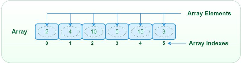
Representation of Array

Arrays support various operations for manipulating their contents:

Accessing Elements: The efficiency of accessing elements in arrays stems from the direct mapping between indices and memory addresses. This mapping allows for constant-time access, as the memory address of any element can be calculated using a simple arithmetic formula involving the base address of the array and the index of the desired element. Indexed access in arrays provides deterministic and efficient retrieval of elements, making arrays suitable for applications requiring rapid data access, such as numerical computations, data processing, and indexing operations.

Creating an array: -
arr = [10, 20, 30, 40, 50]

Accessing elements using indices

print("Element at index 2:", arr[2]) # Output: 30

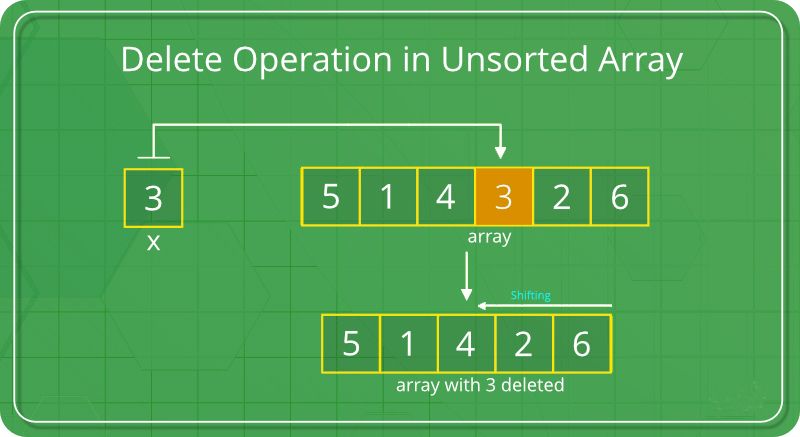
Insertion and Deletion: Insertion and deletion operations in arrays may incur overhead, particularly when performed at arbitrary positions within the array. Insertions and deletions often necessitate shifting subsequent elements to accommodate changes, leading to potential inefficiencies, especially in large arrays. The inefficiency of insertion and deletion operations arises from the need to maintain the contiguous nature of array elements. Insertions and deletions at the beginning or middle of an array may require shifting a significant portion of elements, resulting in increased time complexity proportional to the size of the array.

Insertion at the end of the array: -
arr.append(60)
print("Array after insertion:", arr) # Output: [10, 20, 30, 40, 50, 60]

Deletion at arbitrary position: -
del arr[3]
print("Array after deletion:", arr) # Output: [10, 20, 30, 50, 60]

Traversal: Traversing an array involves iterating over its elements sequentially, typically using loops or iterators. This fundamental operation enables various computational tasks, such as searching, sorting, filtering, and aggregating data stored in the array. Array traversal is essential for performing operations that require accessing or processing each element individually. It allows for efficient data manipulation and analysis, enabling algorithms to operate on the entire dataset stored in the array.

Arrays offer several advantages, including:

Fast Element Access: Arrays provide constant-time access to elements, allowing for rapid retrieval of data based on their indices. This characteristic makes arrays ideal for applications where rapid data access is crucial, such as real-time processing, numerical simulations, and high-performance computing.
Constant-time access ensures predictable performance, regardless of the size of the array or the position of the accessed element, making arrays well-suited for time-sensitive applications where responsiveness is paramount.

Predictable Performance: The fixed size and contiguous memory layout of arrays contribute to their predictable performance characteristics. Arrays exhibit consistent access patterns and memory access times, enabling efficient memory management and access operations. Predictable performance ensures that array operations maintain a consistent time complexity, allowing developers to analyze and optimize algorithms with confidence. This predictability is essential for designing and implementing efficient algorithms and data structures.

Memory Efficiency: Arrays consume memory efficiently, requiring only a single block of contiguous memory to store their elements. This memory layout minimizes memory fragmentation and overhead, resulting in efficient memory utilization and reduced memory footprint. The compact representation of arrays makes them suitable for applications with limited memory resources or stringent memory constraints. Arrays optimize memory usage by eliminating the need for additional metadata or overhead associated with complex data structures.

However, arrays also possess limitations, such as:

Fixed Size: The size of an array is fixed upon creation and cannot be dynamically adjusted at runtime. This limitation restricts their flexibility and may necessitate careful planning when designing applications that require dynamic data storage.

Inefficient Insertion and Deletion: Insertion and deletion operations in arrays may be inefficient, particularly when performed frequently or at arbitrary positions within the array. Shifting elements to accommodate changes can result in additional computational overhead.

Linear search in array: -
def linear_search(arr, target):
for i in range(len(arr)):
if arr[i] == target:
return i
return -1

Example usage: -
index = linear_search(arr, 30)
if index != -1:
print("Element found at index:", index)
else:
print("Element not found")

2. Linked Lists:

Linked lists dynamically allocate memory for elements and use pointers to establish connections between nodes. Singly-linked lists offer efficient insertion and deletion operations at the expense of limited random access, with a time complexity of O(1) for insertion or deletion at the beginning or end, and O(n) for arbitrary positions. Doubly linked lists facilitate bidirectional traversal, but their increased memory overhead results in a space complexity of O(n). Circular linked lists form a circular structure, allowing for continuous traversal without encountering a null reference. However, determining termination conditions and performing operations may introduce complexity.

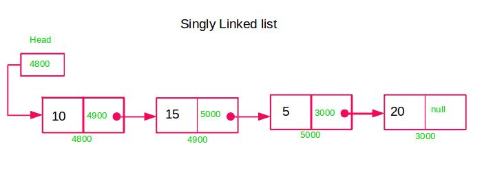
Singly-Linked Lists

Singly-linked lists, a fundamental data structure in computer science, consist of nodes where each node contains a data field and a reference (or pointer) to the next node in the sequence. This structure allows for sequential traversal through the list, starting from the head node and following the next pointers until reaching the end, typically indicated by a null reference. This traversal mechanism enables efficient access to each element in the list, making singly linked lists suitable for scenarios where rapid insertion and deletion operations are common, but random access to elements is not required.

One of the key advantages of singly linked lists is their efficient support for insertion and deletion operations. These operations can be performed swiftly by adjusting the pointers of adjacent nodes, with a time complexity of O(1) when performed at the beginning or end of the list. However, insertions or deletions in the middle of the list may require traversing to the insertion or deletion point, resulting in a time complexity of O(n). Despite this limitation, singly-linked lists remain popular in implementing stacks, queues, and hash tables due to their ability to dynamically resize and manage data efficiently.

Singly-linked lists offer the advantage of dynamic sizing, allowing them to adjust their size dynamically as elements are added to or removed from the list. This flexibility enables efficient memory utilization, as the list can grow or shrink based on the application's requirements without the need for pre-allocation of memory. This dynamic resizing capability is particularly advantageous in scenarios where the number of elements in the list fluctuates frequently, providing adaptive storage management.

From a memory perspective, singly linked lists offer efficient utilization by requiring memory allocation only for the data and pointer fields of each node. This design minimizes memory overhead and facilitates dynamic resizing and management of the list, making it scalable with the number of elements. However, singly-linked lists lack direct access to elements by index, necessitating traversal for specific element retrieval. Moreover, modifications to the list, such as insertion or deletion, require careful management of pointers to prevent memory leaks or data corruption. Thus, thorough testing and validation of list operations are essential to ensure the integrity of the data structure.

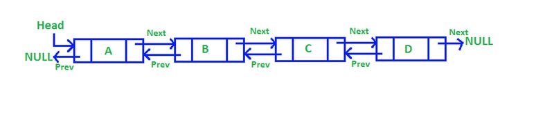
Doubly Linked Lists

Doubly linked lists expand upon the functionality of singly linked lists by incorporating a dual-pointer system in each node, allowing for bidirectional traversal. In addition to pointing to the next node in the sequence, each node in a doubly linked list also contains a pointer to its preceding node. This bidirectional linkage facilitates efficient navigation of the list in both forward and backward directions, enabling versatile data access and manipulation.

These data structures find particular utility in scenarios where bidirectional traversal is essential, such as in the implementation of caches, navigational data structures, and undo mechanisms. Their ability to traverse the list in both directions makes them well-suited for applications requiring rapid access to preceding and succeeding elements.

One of the primary advantages of doubly linked lists is their support for bidirectional traversal. This feature allows for efficient navigation of the list in both forward and backward directions, enhancing the versatility and accessibility of the data structure.

Moreover, insertion and deletion operations within a doubly linked list are efficient, requiring constant time regardless of the position of the operation within the list. This efficiency stems from the list's bidirectional nature, as nodes can be easily inserted or removed without requiring extensive traversal.

Doubly linked lists also offer greater flexibility compared to singly linked lists. Their bidirectional structure enables advanced operations such as reverse traversal and deletion of nodes without requiring knowledge of their predecessors. This flexibility enhances the versatility of doubly linked lists, making them suitable for a wide range of applications.

However, these advantages come with some drawbacks. Doubly linked lists incur increased memory overhead due to the storage of backward pointers in addition to forward pointers. This additional memory requirement can impact the overall memory consumption of the data structure, particularly in scenarios where memory resources are limited.

Furthermore, the implementation of doubly-linked lists is more complex compared to singly-linked lists. Maintaining bidirectional links between nodes increases the complexity of insertion, deletion, and traversal operations, requiring careful management of pointers to ensure the integrity of the list structure. This complexity can lead to challenges in designing and debugging algorithms involving doubly linked lists, necessitating thorough testing and optimization.

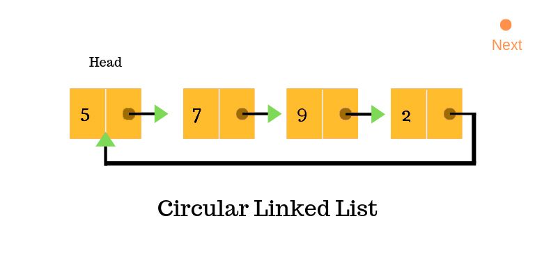
Circular Linked Lists

Circular linked lists constitute a unique variant of linked lists wherein the last node points back to the first node, creating a closed-loop structure. This distinctive arrangement enables continuous traversal of the list without encountering a null reference, simplifying operations that necessitate indefinite iteration over the list.

The circular nature of these lists makes them particularly advantageous in scenarios where cyclic data structures are essential, such as in round-robin scheduling algorithms, circular buffers for resource management, and representing circular paths in graphs.

One significant advantage of circular linked lists lies in their support for continuous traversal without encountering a null reference. This characteristic simplifies certain operations, facilitating seamless iteration over the list without the need for explicit termination conditions.
Additionally, circular linked lists can offer enhanced space efficiency compared to their linear counterparts in specific contexts. By eliminating the requirement for a separate null reference to denote the end of the list, circular linked lists can optimize memory utilization, particularly in scenarios where space constraints are a concern.

However, despite their advantages, circular linked lists also present certain challenges. Determining when to terminate traversal in a circular linked list can be more complex compared to linear lists, as it necessitates additional logic to detect circular loops within the structure. This complexity can complicate algorithm design and debugging, requiring careful consideration of termination conditions to prevent infinite loops.

At the same time, the circular structure introduces increased complexity in operations such as insertion and deletion. Special care must be taken to maintain the integrity of the circular linkage while performing these operations to avoid disrupting the list structure or inadvertently creating infinite loops.
This heightened complexity can pose challenges in implementing and managing circular linked lists, requiring thorough testing and validation to ensure correct behavior.

Operations: Insertion, Deletion, Traversal

Efficient manipulation and traversal of data are essential aspects of working with linked lists. Let's explore the operations of insertion, deletion, and traversal in the context of linked lists:

1. Insertion

Insertion involves adding a new node with a given value into the linked list at a specified position.

Singly-Linked Lists:
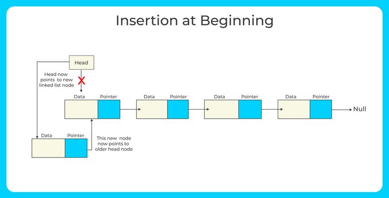
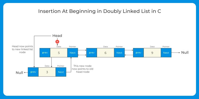
Insertion at the beginning: Create a new node with the desired value and set its next pointer to the current head of the list. Update the head pointer to point to the new node.

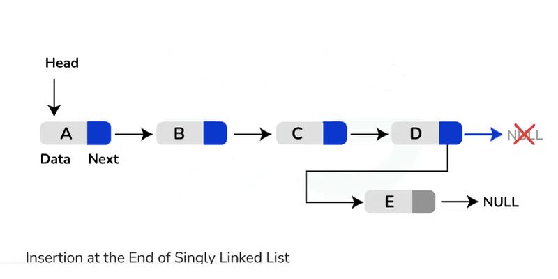
Insertion at the end: Traverse the list until reaching the last node. Create a new node with the desired value and set the next pointer of the last node to point to the new node.

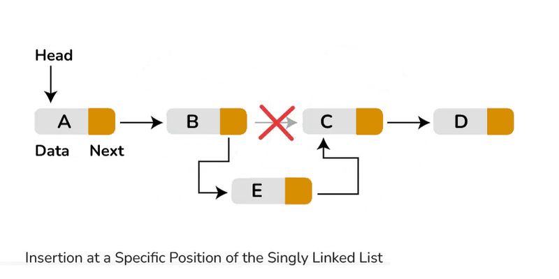
Insertion at a specific position: Traverse the list to the desired position. Create a new node with the desired value, update the next pointer of the previous node to point to the new node, and set the new node's next pointer to the next node in the sequence.

Doubly Linked Lists:

Insertion at the beginning or end: Similar to singly-linked lists, but also update the previous pointer of the previous first or last node, respectively, to point to the new node.

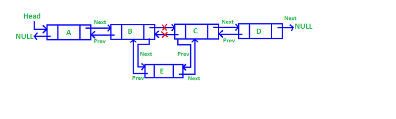
Insertion at a specific position: Traverse the list to the desired position. Create a new node with the desired value, and update the next pointer of the previous node and the previous pointer of the next node to point to the new node.

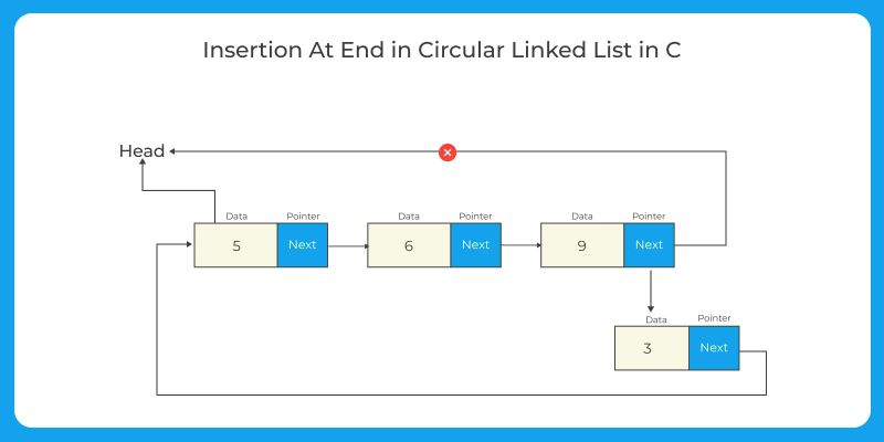
Circular Linked Lists:

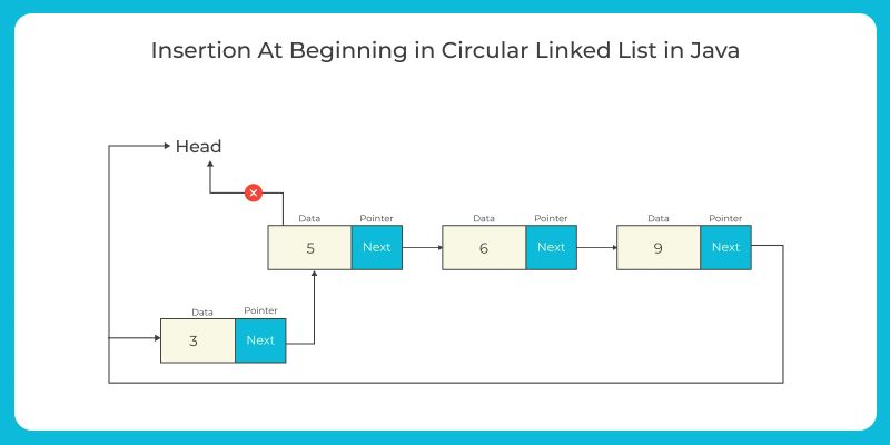
Insertion at the beginning: Similar to singly-linked lists, but update the next pointer of the last node to point to the new node and update the head pointer to point to the new node.

Insertion at the end: Similar to singly-linked lists, but update the next pointer of the last node to point to the new node and update the head pointer to point to the new node.

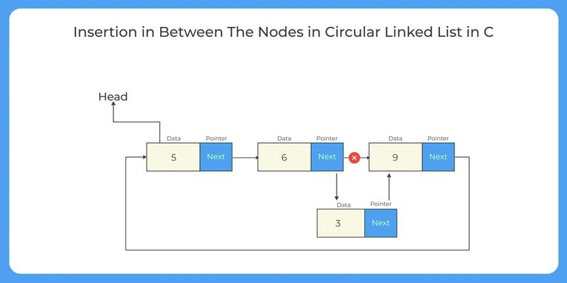
Insertion at a specific position: Traverse the list to the desired position. Create a new node with the desired value, update the next pointer of the previous node to point to the new node, and set the new node's next pointer to the next node in the sequence.

2. Deletion

Deletion involves removing a node with a given value from the linked list.

Singly-Linked Lists:

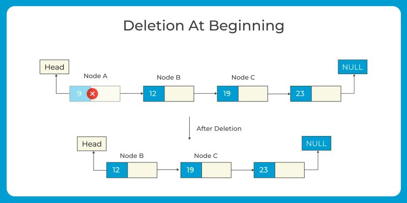
Deletion at the beginning: Update the head pointer to point to the next node in the sequence and free the memory occupied by the deleted node.

Deletion at the end: Traverse the list until reaching the second-to-last node. Update the next pointer of the second-to-last node to point to null and free the memory occupied by the last node.

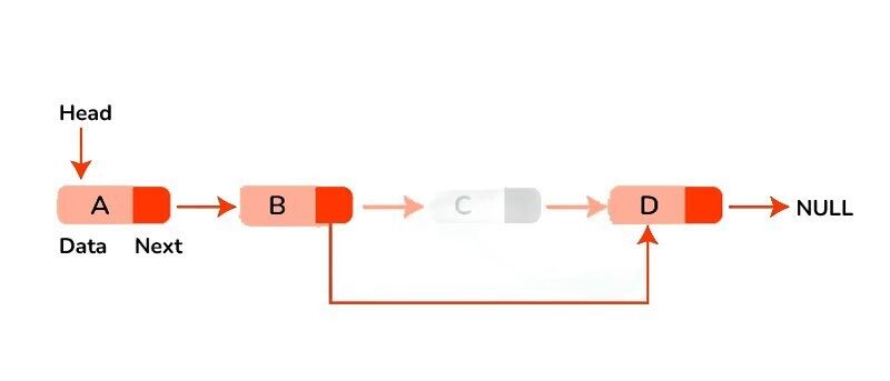
Deletion of a specific value: Traverse the list to find the node with the desired value. Update the next pointer of the previous node to skip over the node to be deleted, and free the memory occupied by the deleted node.

Doubly Linked Lists:

Deletion at the beginning or end: Similar to singly-linked lists, but also update the previous pointer of the new first or last node, respectively, to null.

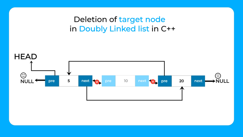
Deletion of a specific value: Similar to singly-linked lists, but also update the previous pointer of the next node and the next pointer of the previous node to bypass the node to be deleted.

Circular Linked Lists:

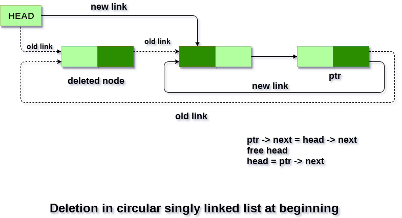
Deletion at the beginning: Similar to singly-linked lists, but update the next pointer of the last node to point to the new first node.

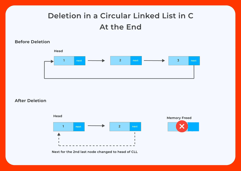
Deletion at the end: Similar to singly-linked lists, but update the next pointer of the second-to-last node to point to the new last node.

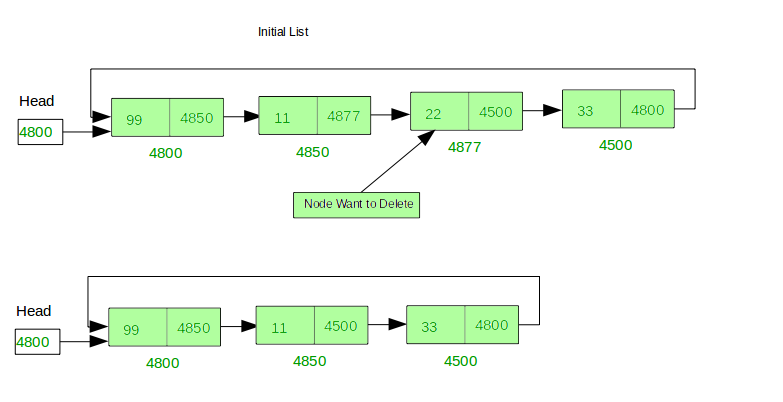
Deletion of a specific value: Similar to singly-linked lists, but also update the next pointer of the previous node and the next pointer of the next node to bypass the node to be deleted.

3. Traversal

Traversal involves visiting each node in the linked list systematically to perform operations or retrieve data.

Singly-Linked Lists, Doubly Linked Lists, Circular Linked Lists:

Forward Traversal: Start from the head (or first) node and iterate through each subsequent node, following the next pointers, until reaching the end of the list.

Backward Traversal (for doubly linked lists only): Start from the tail (or last) node and iterate through each previous node, following the previous pointers, until reaching the beginning of the list.

Circular Traversal (for circular linked lists only): Since circular linked lists do not have a distinct end, traversal can continue indefinitely until a specific condition is met (e.g., reaching the starting point again).

4. Stacks and Queues

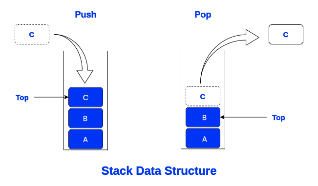
Stacks and queues represent fundamental abstract data types (ADTs) in computer science, serving as versatile tools for managing collections of elements with distinct insertion and removal policies. A stack adheres to the Last In, First Out (LIFO) principle, where the most recently added element is the first to be removed. This linear data structure supports essential operations, including "push," which adds an element to the top of the stack, "pop," which removes and returns the top element, "peek" (or "top"), which retrieves the top element without removing it, and "isEmpty," which checks if the stack is devoid of elements.

Conversely, a queue follows the First In, First Out (FIFO) principle, where the first element inserted is the first to be removed. Operating as a linear data structure, queues offer fundamental operations such as "enqueue," which inserts an element at the rear (end) of the queue, "dequeue," which removes and returns the element from the front (beginning) of the queue, "front," which retrieves the element at the front without dequeuing it, and "isEmpty," which verifies if the queue contains any elements.

Both stacks and queues find extensive use in various applications across computer science and software engineering. Stacks are prevalent in scenarios requiring last-in, first-out access patterns, such as function call management, expression evaluation, and undo mechanisms in text editors.

Conversely, queues are indispensable for managing tasks that demand first-in, first-out behavior, including job scheduling, printer spooling, and message queuing systems in network communication.

In addition to their basic operations, stacks and queues can be implemented using various data structures, such as arrays or linked lists, each offering distinct performance characteristics and trade-offs. Additionally, advanced variations of these ADTs, such as priority queues and double-ended queues (dequeues), provide enhanced functionality for specialized use cases, further highlighting the versatility and utility of stacks and queues in solving a wide range of computational problems.

Implementation and Application of Stacks and Queues

Stacks:

Stacks, a fundamental abstract data type (ADT), find versatile implementations in computer science using arrays or linked lists. While arrays offer constant-time access to elements, their fixed size may limit dynamic resizing capabilities. On the other hand, linked lists provide dynamic resizing capabilities, although they may incur overhead due to pointer manipulation. Stacks play pivotal roles across various applications.

They facilitate expression evaluation by parsing infix, prefix, or postfix notation, enabling efficient arithmetic expression evaluation. Additionally, stacks manage function calls by organizing activation records (stack frames) in recursive function calls, contributing to efficient memory management and control flow. Moreover, stacks serve as indispensable components in implementing undo mechanisms, supporting robust undo functionalities in text editors and software applications.

Furthermore, they enable the implementation of backtracking algorithms, crucial in problem-solving tasks like maze-solving and puzzle games, where efficient exploration of possible solutions is paramount.

Queues:

Queues, another vital ADT, can be realized using arrays, linked lists, or other data structures like circular buffers. Arrays offer constant-time enqueue and dequeue operations, but resizing operations may be required, potentially affecting performance.
Conversely, linked lists facilitate dynamic resizing, albeit with the overhead of pointer manipulation. Queues find widespread application across various domains. They play pivotal roles in job scheduling, managing tasks and processes in operating systems and task schedulers, and ensuring optimal resource allocation and system efficiency.

Additionally, queues facilitate print spooling, efficiently managing print jobs in printers while ensuring equitable access to printing resources for different users. Furthermore, in graph traversal algorithms such as Breadth-First Search (BFS), queues are instrumental in exploring nodes level by level, enabling efficient exploration of graph structures.

Moreover, queues contribute to buffer management in networking protocols and data transmission, handling requests, and managing resources efficiently to ensure seamless data flow and communication.

4. Trees

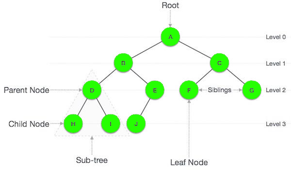
Trees, essential hierarchical data structures, are composed of nodes interconnected by edges, forming a hierarchical arrangement. At the top of the hierarchy stands the root node, from which child nodes extend. Each node can have zero or more child nodes, establishing a parent-child relationship. Unlike linear data structures, trees offer hierarchical organization, facilitating efficient representation and manipulation of relationships.

In addition to the root node, trees comprise internal nodes and leaf nodes. Internal nodes connect child nodes, while leaf nodes, at the lowest levels, lack child nodes. This structure enables trees to model various hierarchical relationships encountered in real-world scenarios, which is vital across computer science, data management, and artificial intelligence.

In computer science, trees are pivotal in data storage and retrieval operations, enabling efficient searching, sorting, and indexing. Binary search trees (BSTs) ensure rapid searching and insertion by maintaining a sorted hierarchy. They organize and structure data hierarchically in data management, facilitating storage and retrieval. Hierarchical data models, like XML and JSON, leverage trees for complex data relationships.

In artificial intelligence, trees power decision-making systems like decision trees and game trees, facilitating efficient decision-making and strategic planning. Decision trees automate decisions based on input features, while game trees model moves and outcomes in strategic games. Trees, with their hierarchical nature and traversal algorithms, are indispensable across a broad spectrum of applications.

Let's now explore three important types of trees:

Binary Trees:

Binary trees represent a foundational concept in computer science, embodying a hierarchical data structure composed of nodes interconnected through edges. Within this structure, each node can have at most two children, known as the left child and the right child, facilitating efficient data organization and retrieval. Beyond their theoretical significance, binary trees find practical application in diverse fields, notably in decision tree models employed for decision-making processes across finance, healthcare, and engineering domains. Decision trees, a type of binary tree, enable systematic analysis by representing decision paths based on specific criteria or attributes, aiding in scenarios like stock price predictions in finance, disease diagnosis in healthcare, and fault diagnosis in engineering systems. In essence, binary trees not only underpin fundamental concepts in computer science but also offer tangible benefits in real-world problem-solving contexts.

class TreeNode:
def init(self, value):
self.value = value
self.left = None
self.right = None

Example usage of binary tree node

root = TreeNode(10)
root.left = TreeNode(5)
root.right = TreeNode(15)

Binary Search Trees (BST):

Binary search trees serve as a fundamental data structure in software engineering and database management, offering efficient search, insertion, and deletion operations. Their unique property of maintaining ordered nodes facilitates fast searching algorithms, leading to applications such as symbol tables in compilers and dictionaries in programming languages. Symbol tables, implemented using binary search trees, store information about identifiers and their attributes, optimizing compilation processes and program execution. Additionally, binary search trees find application in real-world scenarios such as dictionary implementations in software libraries, enabling rapid retrieval and manipulation of key-value pairs. Thus, beyond their theoretical elegance, binary search trees contribute to practical software development, enhancing efficiency and performance in diverse applications.

class TreeNode:
def init(self, key, value):
self.key = key
self.value = value
self.left = None
self.right = None

class BST:
def init(self):
self.root = None

def insert(self, key, value):
    self.root = self._insert(self.root, key, value)

def _insert(self, node, key, value):
    if node is None:
        return TreeNode(key, value)
    if key < node.key:
        node.left = self._insert(node.left, key, value)
    elif key > node.key:
        node.right = self._insert(node.right, key, value)
    return node

Example usage of binary search tree

bst = BST()
bst.insert(10, 'A')
bst.insert(5, 'B')
bst.insert(15, 'C')

AVL Trees:
AVL trees represent a specialized form of self-balancing binary search trees, ensuring logarithmic time complexity for search, insertion, and deletion operations. This balance property, coupled with predictable performance characteristics, makes AVL trees indispensable in critical domains such as finance. In banking systems, AVL trees facilitate efficient transaction processing, maintaining account balances and managing customer portfolios with accuracy and timeliness. Similarly, in investment and trading platforms, AVL trees enable real-time data management, supporting rapid retrieval of market information and execution of trades. Moreover, AVL trees play a crucial role in database indexing structures, ensuring consistent performance and rapid data retrieval in large-scale applications. In summary, AVL trees not only provide theoretical elegance but also offer practical solutions for managing and processing vast volumes of data in real-world scenarios.
class AVLTreeNode:
def init(self, key, value):
self.key = key
self.value = value
self.left = None
self.right = None
self.height = 1

class AVLTree:
def init(self):
self.root = None

def insert(self, key, value):
    self.root = self._insert(self.root, key, value)

def _insert(self, node, key, value):
    if node is None:
        return AVLTreeNode(key, value)
    if key < node.key:
        node.left = self._insert(node.left, key, value)
    elif key > node.key:
        node.right = self._insert(node.right, key, value)
    else:
        return node

    node.height = 1 + max(self._get_height(node.left), self._get_height(node.right))
    balance = self._get_balance(node)

    # Left Left Case
    if balance > 1 and key < node.left.key:
        return self._right_rotate(node)

    # Right Right Case
    if balance < -1 and key > node.right.key:
        return self._left_rotate(node)

    # Left Right Case
    if balance > 1 and key > node.left.key:
        node.left = self._left_rotate(node.left)
        return self._right_rotate(node)

    # Right Left Case
    if balance < -1 and key < node.right.key:
        node.right = self._right_rotate(node.right)
        return self._left_rotate(node)

    return node

def _get_height(self, node):
    if node is None:
        return 0
    return node.height

def _get_balance(self, node):
    if node is None:
        return 0
    return self._get_height(node.left) - self._get_height(node.right)

def _left_rotate(self, z):
    y = z.right
    T2 = y.left

    y.left = z
    z.right = T2

    z.height = 1 + max(self._get_height(z.left), self._get_height(z.right))
    y.height = 1 + max(self._get_height(y.left), self._get_height(y.right))

    return y

def _right_rotate(self, y):
    x = y.left
    T2 = x.right

    x.right = y
    y.left = T2

    y.height = 1 + max(self._get_height(y.left), self._get_height(y.right))
    x.height = 1 + max(self._get_height(x.left), self._get_height(x.right))

    return x

Example usage of AVL tree

avl_tree = AVLTree()
avl_tree.insert(10, 'A')
avl_tree.insert(5, 'B')
avl_tree.insert(15, 'C')

5. Graphs

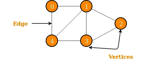
Graphs are versatile data structures used to represent relationships between objects. A graph is generally denoted as a collection of vertices and edges, where edges represent relationships or connections between pairs of vertices. There are two types of graphs: a directed graph or digraph, and an undirected graph.

In a directed graph, edges have a direction associated with them. They indicate a one-way relationship between vertices. Whereas, in an undirected graph, edges do not have a direction. They represent symmetric relationships between vertices, where each edge connects two vertices bidirectionally.

Representations for Storing Graph Data

The Adjacency Matrix and the Adjacency List are the two commonly used representations for storing graph data.
An adjacency matrix is essentially a 2D array where each cell (i, j) indicates whether there exists an edge between vertex i and vertex j. For undirected graphs, this matrix exhibits symmetry across the main diagonal. While adjacency matrices excel in efficiently retrieving edge information in dense graphs, providing constant-time lookup, they consume considerable memory for sparse graphs due to their quadratic space complexity.

On the other hand, an adjacency list is a collection of lists or arrays, where each vertex maintains a list of its adjacent vertices. This approach requires less memory for sparse graphs, as each vertex's adjacency list only stores references to its neighboring vertices. However, edge lookup operations in adjacency lists can be slower compared to adjacency matrices, with varying time complexities for different operations.

Despite their differences, both representations serve distinct purposes, catering to different graph characteristics and computational requirements.

Graph Traversal Algorithms

Depth-First Search (DFS) and Breadth-First Search (BFS) are the two fundamental techniques for exploring the structure of a graph and analyzing its properties. DFS operates by systematically traversing along each branch as deeply as possible before backtracking, effectively exploring the graph's depth-first nature. Employing a stack, either explicitly or implicitly through recursion, DFS maintains the traversal path, making it well-suited for tasks such as topological sorting, cycle detection, maze solving, and identifying graph components.

In contrast, BFS explores the graph by systematically traversing all vertices at the current depth level before moving on to the next level. By utilizing a queue to manage the traversal order, BFS ensures that vertices are visited in the order they were discovered, making it ideal for applications such as finding shortest paths, network broadcasting, and performing level-order traversal in trees.

These traversal algorithms play pivotal roles in various domains, facilitating efficient exploration and analysis of graph structures and enabling the development of diverse graph-based applications.

Understanding Algorithms

Algorithms form the backbone of computer science, providing systematic approaches to solving computational problems efficiently. Understanding algorithms involves delving into various categories, including Sorting Algorithms, Searching Algorithms, Dynamic Programming, and Greedy Algorithms.

Sorting Algorithms:
Sorting algorithms are fundamental algorithms used to arrange a collection of elements in a specific order, typically ascending or descending. These algorithms play a crucial role in various applications, such as data processing, searching, and optimization.
Here's an overview of some common sorting algorithms:

Bubble Sort:
Bubble sort is a simple sorting algorithm that repeatedly steps through the list, compares adjacent elements, and swaps them if they are in the wrong order. This process continues until the entire list is sorted.
While bubble sort is easy to understand and implement, it is relatively inefficient for large datasets due to its quadratic time complexity.

Bubble Sort Code

def bubble_sort(arr):
n = len(arr)
for i in range(n-1):
for j in range(0, n-i-1):
if arr[j] > arr[j+1]:
arr[j], arr[j+1] = arr[j+1], arr[j]

Selection Sort:
Selection sort divides the input list into two parts: a sorted sublist and an unsorted sublist. The algorithm repeatedly finds the minimum (or maximum) element from the unsorted sublist and swaps it with the first element of the unsorted sublist.

This process continues until the entire list is sorted. Although selection sort is simple and performs well for small datasets, it has a time complexity of O(n^2), making it inefficient for large lists.

Selection Sort Code

def selection_sort(arr):
n = len(arr)
for i in range(n):
min_idx = i
for j in range(i+1, n):
if arr[j] < arr[min_idx]:
min_idx = j
arr[i], arr[min_idx] = arr[min_idx], arr[i]
return arr

Example usage:

arr = [64, 25, 12, 22, 11]
sorted_arr = selection_sort(arr)
print("Sorted array:", sorted_arr)

Insertion Sort:
Insertion sort builds the final sorted array one element at a time by repeatedly taking the next element from the unsorted part of the array and inserting it into its correct position in the sorted part of the array. It is efficient for small datasets and nearly sorted lists but becomes inefficient for large datasets due to its quadratic time complexity.

Insertion Sort Code

def insertion_sort(arr):
for i in range(1, len(arr)):
key = arr[i]
j = i - 1
while j >= 0 and key < arr[j]:
arr[j + 1] = arr[j]
j -= 1
arr[j + 1] = key

Merge Sort:
Merge sort is a divide-and-conquer algorithm that recursively divides the input array into smaller subarrays until each subarray contains only one element. It then merges these subarrays in a sorted order until the entire array is sorted. Merge sort is efficient and stable, with a time complexity of O(n log n), making it suitable for sorting large datasets.

Merge Sort Code

def merge_sort(arr):
if len(arr) > 1:
mid = len(arr) // 2
L = arr[:mid]
R = arr[mid:]

    merge_sort(L)
    merge_sort(R)

    i = j = k = 0

    while i < len(L) and j < len(R):
        if L[i] < R[j]:
            arr[k] = L[i]
            i += 1
        else:
            arr[k] = R[j]
            j += 1
        k += 1

    while i < len(L):
        arr[k] = L[i]
        i += 1
        k += 1

    while j < len(R):
        arr[k] = R[j]
        j += 1
        k += 1

return arr

Example usage:

arr = [64, 25, 12, 22, 11]
sorted_arr = merge_sort(arr)
print("Sorted array:", sorted_arr)

Quick Sort:
Quick sort is another divide-and-conquer algorithm that partitions the input array into two subarrays based on a pivot element. It then recursively sorts the subarrays and combines them to form the final sorted array.

Quick sort is efficient and widely used, with an average time complexity of O(n log n). However, its worst-case time complexity of O(n^2) can occur when the pivot selection is poor.

Quick Sort Code

def quick_sort(arr):
if len(arr) <= 1:
return arr
pivot = arr[len(arr) // 2]
left = [x for x in arr if x < pivot]
middle = [x for x in arr if x == pivot]
right = [x for x in arr if x > pivot]
return quick_sort(left) + middle + quick_sort(right)

Example usage:

arr = [64, 25, 12, 22, 11]
sorted_arr = quick_sort(arr)
print("Sorted array:", sorted_arr)

2. Searching Algorithms

Searching algorithms are essential tools in computer science, enabling efficient retrieval of specific elements within data collections. They play a critical role in various applications, ranging from database queries to information retrieval systems. These algorithms can be broadly categorized into two main types: sequential search and binary search.

Sequential search, also known as linear search, involves scanning through each element in a list or array one by one until the desired element is found. While simple to implement, sequential search may become inefficient for large datasets, as its time complexity is directly proportional to the size of the dataset, with a worst-case time complexity of O(n), where n is the number of elements in the list.

In contrast, binary search is a more efficient algorithm for searching in sorted arrays. It follows a divide-and-conquer approach, repeatedly dividing the search interval in half until the target element is found or the search interval is empty. Binary search achieves a time complexity of O(log n), making it significantly faster than sequential search for large datasets.

Apart from these basic searching algorithms, hashing and hash tables provide an alternative approach to searching. Hashing involves mapping data elements to fixed-size values using hash functions, which are then stored in hash tables. Hash tables offer constant-time average-case performance for insertion, deletion, and lookup operations, making them highly efficient for searching.

However, collisions, where multiple elements map to the same hash value, may occur, necessitating collision resolution techniques such as chaining or open addressing.

Linear Search Code

def linear_search(arr, target):
for i in range(len(arr)):
if arr[i] == target:
return i
return -1

Binary Search Code (Assumes the input list is sorted)
def binary_search(arr, target):
low, high = 0, len(arr) - 1
while low <= high:
mid = (low + high) // 2
if arr[mid] == target:
return mid
elif arr[mid] < target:
low = mid + 1
else:
high = mid - 1
return -1

3. Dynamic Programming

Dynamic programming is a powerful technique in computer science and mathematics for solving optimization problems by breaking them down into smaller subproblems and solving each subproblem only once. This approach significantly reduces redundant computations and improves the efficiency of algorithms.

The concept of dynamic programming revolves around two main principles: overlapping subproblems and optimal substructure. Overlapping subproblems refer to instances where the same subproblems recur multiple times during the computation, while optimal substructure implies that the optimal solution to a problem can be constructed from the optimal solutions of its subproblems.

One classic example that illustrates dynamic programming is the Fibonacci series. In this sequence, each number is the sum of the two preceding ones, starting from 0 and 1. While a naive recursive approach to computing Fibonacci numbers may lead to redundant calculations, dynamic programming techniques such as memoization or tabulation can efficiently compute Fibonacci numbers by storing the results of subproblems and reusing them as needed.

Another well-known problem often tackled using dynamic programming is the Knapsack problem, which involves selecting a subset of items with maximum value while ensuring that their total weight does not exceed a given limit. By breaking down the problem into smaller subproblems, dynamic programming algorithms can efficiently explore different combinations of items and determine the optimal solution.

Memoization and tabulation are two common approaches used in dynamic programming to store and reuse intermediate results. Memoization involves storing the results of subproblems in a data structure, such as a dictionary or an array, to avoid redundant computations during recursion.
On the other hand, tabulation involves building a table or matrix to store the results of subproblems iteratively, typically using bottom-up dynamic programming. Both techniques offer advantages depending on the problem at hand, with memoization being more intuitive for recursive algorithms and tabulation offering better performance and space efficiency for iterative algorithms.

Using the memoization technique for Fibonacci series

def fibonacci_memo(n, memo={}):
if n in memo:
return memo[n]
if n <= 1:
return n
memo[n] = fibonacci_memo(n - 1, memo) + fibonacci_memo(n - 2, memo)
return memo[n]

Example usage:

n = 10
print("Fibonacci sequence using memoization:")
for i in range(n):
print(fibonacci_memo(i), end=" ")
print()

Using tabulation technique for Fibonacci series

def fibonacci_tab(n):
if n <= 1:
return n
fib = [0] * (n + 1)
fib[1] = 1
for i in range(2, n + 1):
fib[i] = fib[i - 1] + fib[i - 2]
return fib[n]

Example usage:

print("\nFibonacci sequence using tabulation:")
for i in range(n):
print(fibonacci_tab(i), end=" ")
print()

4. Greedy Algorithms

Greedy algorithms are problem-solving strategies that make locally optimal choices at each step in the hope of finding a globally optimum solution. These algorithms focus on immediate gains without considering future consequences, resulting in solutions that may not always be globally optimal. Despite this limitation, greedy algorithms are characterized by their simplicity and efficiency, as they typically require fewer computational resources compared to other techniques like dynamic programming.

One classic example of a greedy algorithm is the Minimum Spanning Tree (MST) problem, where the objective is to find the minimum weight-connected subgraph that spans all vertices in a given graph.
Kruskal's algorithm and Prim's algorithm are commonly used greedy approaches to solve this problem, each iteratively selecting edges based on their weights to grow the minimum spanning tree.

Another example of a greedy algorithm is Huffman coding, which is used for lossless data compression. Huffman coding assigns variable-length prefix-free codes to characters in the input data based on their frequencies, with more frequent characters receiving shorter codes. By iteratively merging the least frequent characters into a binary tree, Huffman coding constructs an optimal prefix-free code that achieves efficient data compression without loss of information.

Despite their simplicity and efficiency, it's important to note that greedy algorithms may not always yield the optimal solution for every problem and may produce suboptimal results in some cases. However, they remain valuable problem-solving tools and have applications in various domains, including network routing, scheduling, and data compression.

Huffman Coding Example

from heapq import heappush, heappop, heapify
from collections import defaultdict

def huffman_encoding(data):
freq = defaultdict(int)
for char in data:
freq[char] += 1

heap = [[weight, [symbol, ""]] for symbol, weight in freq.items()]
heapify(heap)

while len(heap) > 1:
    lo = heappop(heap)
    hi = heappop(heap)
    for pair in lo[1:]:
        pair[1] = '0' + pair[1]
    for pair in hi[1:]:
        pair[1] = '1' + pair[1]
    heappush(heap, [lo[0] + hi[0]] + lo[1:] + hi[1:])

return heap[0][1]

def huffman_decoding(data, tree):
result = ""
current = tree
for bit in data:
if bit == '0':
current = current[0]
else:
current = current[1]
if type(current) is tuple:
result += current[0]
current = tree
return result

Practical Applications

Data structures and algorithms play a vital role in various real-world scenarios, spanning software development, system design, and problem-solving. Here are some examples demonstrating their use:

Database Management Systems (DBMS):

Database Management Systems rely heavily on data structures and algorithms to efficiently store, retrieve, and manipulate large volumes of data. Data structures like B-trees and hash tables are commonly used for indexing and organizing data, while algorithms such as binary search and hashing optimize data retrieval operations.

Additionally, query optimization techniques employ algorithms to analyze and optimize the execution of complex database queries, enhancing performance and scalability.

Network Routing Algorithms:

In computer networks, routing algorithms determine the optimal paths for data packets to travel from source to destination. Data structures such as graphs are used to model network topologies, while algorithms like Dijkstra's algorithm and Bellman-Ford algorithm compute the shortest paths between nodes.
These algorithms play a crucial role in ensuring efficient data transmission, minimizing latency, and maximizing network throughput.

Machine Learning and Artificial Intelligence (AI):

Machine learning and AI algorithms heavily rely on data structures for representing and processing large datasets. Data structures like arrays, matrices, and graphs are used to store and manipulate input data, while algorithms such as neural networks, decision trees, and clustering algorithms analyze and extract patterns from the data.
These techniques find applications in various domains, including image recognition, natural language processing, and recommendation systems.

System Design and Optimization:

Data structures and algorithms are essential components in designing scalable and efficient systems. For example, designing caching systems using data structures like LRU (Least Recently Used) cache or LFU (Least Frequently Used) cache algorithms can significantly improve system performance by reducing data access latency.

Similarly, load-balancing algorithms distribute incoming traffic across multiple servers to optimize resource utilization and ensure high availability.

Algorithmic Trading:

In financial markets, algorithmic trading relies on sophisticated algorithms and data structures to analyze market data, execute trades, and manage risk. Data structures like priority queues and hash tables are used to store and process market data, while algorithms such as arbitrage algorithms and trend-following strategies automate trading decisions based on predefined rules and market conditions.

Genetic Algorithms in Optimization:

Genetic algorithms, inspired by the process of natural selection, are used in optimization problems to find optimal solutions in complex search spaces. These algorithms employ data structures like chromosomes and populations to represent potential solutions and evolve them over generations using genetic operators like mutation and crossover.

Genetic algorithms find applications in diverse fields, including engineering design, scheduling, and evolutionary biology.

Conclusion

Data structures and algorithms are the backbone of computer science and software development, providing systematic approaches to organizing, processing, and analyzing data efficiently. From arrays and linked lists to trees and graphs, each structure offers unique advantages for solving computational problems. Coupled with algorithms like sorting, searching, and dynamic programming, these tools empower developers to tackle complex challenges and optimize system performance.

From the efficient manipulation of arrays to the dynamic nature of linked lists, and from the hierarchical organization of trees to the versatile representation of graphs, these data structures form the backbone of countless applications across diverse domains. Moreover, the accompanying algorithms, ranging from sorting and searching to dynamic programming and greedy strategies, equip developers with powerful tools for solving complex computational problems and optimizing system performance.

In practical scenarios, data structures and algorithms find widespread applications, from database management systems and network routing algorithms to machine learning and artificial intelligence techniques. Whether it's optimizing query execution in a database, ensuring efficient data transmission in a network, or automating trading decisions in financial markets, the role of data structures and algorithms is indispensable in shaping the modern technological landscape.

In essence, data structures and algorithms form the bedrock of computational thinking, empowering developers to navigate the complexities of modern computing and innovate solutions that drive progress in an increasingly digital world. As technology continues to evolve, the importance of a holistic understanding of data structures and algorithms remains paramount, ensuring that developers can leverage their capabilities to tackle emerging challenges and drive innovation forward.